{"name":"domb-napari","display_name":"DoMB","visibility":"public","icon":"","categories":["Image Processing","Segmentation","Utilities"],"schema_version":"0.2.1","on_activate":null,"on_deactivate":null,"contributions":{"commands":[{"id":"domb-napari.split_channels_widget","title":"Multichannel stack preprocessing","python_name":"domb_napari._widget:split_channels","short_title":null,"category":null,"icon":null,"enablement":null},{"id":"domb-napari.dw_registration_widget","title":"Dual-view stack registration","python_name":"domb_napari._widget:dw_registration","short_title":null,"category":null,"icon":null,"enablement":null},{"id":"domb-napari.cross_calc_widget","title":"E-FRET crosstalk estimation","python_name":"domb_napari._widget:cross_calc","short_title":null,"category":null,"icon":null,"enablement":null},{"id":"domb-napari.g_calc_widget","title":"E-FRET G-factor estimation","python_name":"domb_napari._widget:g_calc","short_title":null,"category":null,"icon":null,"enablement":null},{"id":"domb-napari.e_app_widget","title":"E-FRET estimation","python_name":"domb_napari._widget:e_app_calc","short_title":null,"category":null,"icon":null,"enablement":null},{"id":"domb-napari.der_series_widget","title":"Red-green series","python_name":"domb_napari._widget:der_series","short_title":null,"category":null,"icon":null,"enablement":null},{"id":"domb-napari.up_mask_calc_widget","title":"Up masking","python_name":"domb_napari._widget:up_mask_calc","short_title":null,"category":null,"icon":null,"enablement":null},{"id":"domb-napari.mask_calc_widget","title":"Intensity masking","python_name":"domb_napari._widget:mask_calc","short_title":null,"category":null,"icon":null,"enablement":null},{"id":"domb-napari.labels_profiles_set_widget","title":"ROIs profiles","python_name":"domb_napari._widget:labels_profile_line","short_title":null,"category":null,"icon":null,"enablement":null},{"id":"domb-napari.labels_multi_profile_widget","title":"Multiple img stat profiles","python_name":"domb_napari._widget:labels_multi_profile_stat","short_title":null,"category":null,"icon":null,"enablement":null},{"id":"domb-napari.multi_labels_profile_widget","title":"Multiple labels stat profiles","python_name":"domb_napari._widget:multi_labels_profile_stat","short_title":null,"category":null,"icon":null,"enablement":null},{"id":"domb-napari.dot_mask_widget","title":"Dot-patterns masking","python_name":"domb_napari._widget:dot_mask_calc","short_title":null,"category":null,"icon":null,"enablement":null},{"id":"domb-napari.save_df_widget","title":"Save Data Frame","python_name":"domb_napari._widget:save_df","short_title":null,"category":null,"icon":null,"enablement":null},{"id":"domb-napari.rel_series_widget","title":"ΔF series","python_name":"domb_napari._widget:rel_series","short_title":null,"category":null,"icon":null,"enablement":null}],"readers":null,"writers":null,"widgets":[{"command":"domb-napari.dw_registration_widget","display_name":"Dual-view stack registration","autogenerate":false},{"command":"domb-napari.split_channels_widget","display_name":"Multichannel stack preprocessing","autogenerate":false},{"command":"domb-napari.der_series_widget","display_name":"Red-green series","autogenerate":false},{"command":"domb-napari.rel_series_widget","display_name":"ΔF series","autogenerate":false},{"command":"domb-napari.e_app_widget","display_name":"FRET estimation","autogenerate":false},{"command":"domb-napari.cross_calc_widget","display_name":"FRET cross-talk estimation","autogenerate":false},{"command":"domb-napari.g_calc_widget","display_name":"FRET G-factor estimation","autogenerate":false},{"command":"domb-napari.dot_mask_widget","display_name":"Dot-patterns masking","autogenerate":false},{"command":"domb-napari.up_mask_calc_widget","display_name":"Up masking","autogenerate":false},{"command":"domb-napari.mask_calc_widget","display_name":"Intensity masking","autogenerate":false},{"command":"domb-napari.labels_profiles_set_widget","display_name":"ROIs profiles","autogenerate":false},{"command":"domb-napari.labels_multi_profile_widget","display_name":"Multiple img stat profiles","autogenerate":false},{"command":"domb-napari.multi_labels_profile_widget","display_name":"Multiple labels stat profiles","autogenerate":false},{"command":"domb-napari.save_df_widget","display_name":"Save Data Frame","autogenerate":false}],"sample_data":null,"themes":null,"menus":{"napari/layers/visualize":[{"when":null,"group":null,"submenu":"profiles"}],"profiles":[{"command":"domb-napari.labels_profiles_set_widget","when":null,"group":null,"alt":null},{"command":"domb-napari.labels_multi_profile_widget","when":null,"group":null,"alt":null},{"command":"domb-napari.multi_labels_profile_widget","when":null,"group":null,"alt":null}],"napari/layers/data":[{"when":null,"group":null,"submenu":"preprocessing"},{"command":"domb-napari.save_df_widget","when":null,"group":null,"alt":null}],"preprocessing":[{"command":"domb-napari.split_channels_widget","when":null,"group":null,"alt":null},{"command":"domb-napari.dw_registration_widget","when":null,"group":null,"alt":null}],"napari/layers/measure":[{"command":"domb-napari.der_series_widget","when":null,"group":null,"alt":null},{"command":"domb-napari.rel_series_widget","when":null,"group":null,"alt":null},{"when":null,"group":null,"submenu":"e-fret"}],"e-fret":[{"command":"domb-napari.e_app_widget","when":null,"group":null,"alt":null},{"command":"domb-napari.g_calc_widget","when":null,"group":null,"alt":null},{"command":"domb-napari.cross_calc_widget","when":null,"group":null,"alt":null}],"napari/layers/segment":[{"command":"domb-napari.dot_mask_widget","when":null,"group":null,"alt":null},{"command":"domb-napari.up_mask_calc_widget","when":null,"group":null,"alt":null},{"command":"domb-napari.mask_calc_widget","when":null,"group":null,"alt":null}]},"submenus":[{"id":"e-fret","label":"FRET","icon":null},{"id":"profiles","label":"Labels Profiles","icon":null},{"id":"preprocessing","label":"Preprocessing","icon":null}],"keybindings":null,"configuration":[]},"package_metadata":{"metadata_version":"2.4","name":"domb-napari","version":"0.5.2","dynamic":["license-file"],"platform":null,"supported_platform":null,"summary":"napari plugin for analyzing the redistribution of fluorescence-labeled proteins","description":"domb-napari\n===========\n\n[](https://stand-with-ukraine.pp.ua)\n\n[](https://napari-hub.org/plugins/domb-napari)\n\n\n[](https://doi.org/10.5281/zenodo.14843770)\n\n\n__napari Toolkit of Department of Molecular Biophysics
Bogomoletz Institute of Physiology of NAS of Ukraine, Kyiv, Ukraine__\n\nThis plugin offers widgets specifically designed to analyze the redistribution of fluorescence-labeled proteins in widefield epifluorescence time-lapse acquisitions. It is particularly useful for studying various phenomena, including:\n- Calcium-dependent translocation of neuronal calcium sensors.\n- Synaptic receptor traffic.\n- Membrane protein tracking.\n\n\n__Hippocalcin (neuronal calcium sensor) redistributes in dendritic branches upon NMDA application__\n\n### Plugin Menus\nThe plugin widgets are distributed across the following napari `Layers` menus:\n\n- **Visualize**\n - `Labels Profiles` submenu: _ROIs profiles_, _Multiple img stat profiles_, _Multiple labels stat profiles_\n- **Data**\n - `Preprocessing` submenu: _Multichannel stack preprocessing_, _Dual-view stack registration_\n - _Save Data Frame_\n- **Measure**\n - _Red-green series_\n - _ΔF series_\n - `FRET` submenu: _E-FRET estimation_, _E-FRET G-factor estimation_, _E-FRET crosstalk estimation_\n- **Segment**\n - _Dot-patterns masking_\n - _Up masking_\n - _Intensity masking_\n\n### Plugin Structure\n``` mermaid\ngraph TD\n \nsubgraph Preprocessing [Preprocessing]\n MP[Multichannel Image Preprocessing]\n R[Multichannel Image Registration]\n\tR --> MP\nend\n\nsubgraph Analysis [Analysis]\n DF[ΔF Series]\n RG[Red-green Series]\nend\nMP ==> Analysis\n\nsubgraph FRET [FRET]\n\tsubgraph Calibration [Calibration]\n FC[Cross-talk Estimation]\n FG[G-factor Estimation]\n end\n FR[FRET Estimation]\n \nend\nMP ==> FRET\nFR ---> Analysis\nFR ---> Segmentation\n\n\n\nsubgraph Segmentation [Segmentation]\n UP[Up Masking]\n DOWN[Masking]\n DOT[Dot-pattern Masking]\nend\n%% MP ==> Segmentation\nAnalysis ==> Segmentation\n\n\nsubgraph Vis [Visualization & Data Saving]\n subgraph Stat [Aggregated Plots]\n MIP[Multiple Images Profiles]\n MMP[Multiple Masks Profiles]\n end\n RP[ROIs Profiles]\n DAT[Data Frame Saving]\nend\nSegmentation ==> Vis\nFRET ==> Vis\n\n```\n\n\n### E-FRET Module Structure\n``` mermaid\nflowchart TD\n %% INPUT DATA\n %% Input[/Input Images:
IDD, IDA, IAA/]:::data\n Input@{shape: manual-input, label: \"Input Images:
IDD, IDA, IAA\"}\n \n %% Mask[/ROIs Mask/]:::data\n Mask@{shape: manual-input, label: \"ROIs Mask\"}\n\n %% CALIBRATION\n subgraph Calibration [Coefficients Estimation]\n %% direction TB\n \n CT[_CrossTalkEstimation_ Class]:::algo\n GF[_GFactorEstimation_ Class]:::algo\n \n Coeffs(Cross-talk coefs. __a__ & __d__):::result\n GF_Val(__G__ factor):::result\n\n Input -->|Samples with A or D only| CT\n Mask --> CT\n CT -->|Linear regression| Coeffs\n \n Input -->|Samples with AD tandem| GF\n Mask & Coeffs --> GF\n GF -->|Zal / Chen method| GF_Val\n end\n\n %% ANA\n subgraph Analysis [FRET Estimation]\n %% direction TB\n \n Main[_CubesFRET_ Class]:::algo\n Numba[[JIT compiled Numba functions]]:::algo\n Output(Pixel-wise FRET estimation:
Fc, ED, EA, Ecorr):::result\n\n Input ==> Main\n Coeffs & GF_Val ==> Main\n \n Main ==> Output\n Main <-...->|Pixel-wise calc| Numba\n end\n```\n\n---\n\n## Preprocessing\n### Dual-view Stack Registration\nRegistration of four-channel image stacks, including two excitation wavelengths and two emission pathbands, acquired with a dual-view beam splitter. This setup detects different spectral pathbands using distinct sides of the camera matrix.\n\n- `offset img` - input for a four-channel time-lapse image stack.\n- `input crop` - number of pixels to remove from each side of input frames to eliminate beam-splitter alignment artifacts.\n- `output crop` - number of pixels to remove from each side of output frames to eliminate registration edge artifacts.\n- `align method` - choice between:\n - `internal` - automated registration based on the input stack.\n - `load matrix` - applies a pre-calculated affine transformation matrix from a `.txt` file.\n- `manual channels` - enables manual selection of Reference and Offset channels for registration.\n- `ref_off_ch` - defines which spectral channels to use for offset estimation.\n- `save matrix` - exports the calculated affine transformation matrix to a `.txt` file at the specified `saving path`.\n\n\n### Multichannel Stack Preprocessing\n- `stack order` - specifies the axis order of the input data: T (time), C (channel), X, and Y.\n- `median filter` - applies frame-by-frame smoothing with a kernel size specified in `median kernel`.\n- `background subtraction` - compensates for background fluorescence. The background is estimated as the 1.0 percentile of frame intensity.\n- `photobleaching correction` - fits the total intensity decay using exponential (`exp`) or bi-exponential (`bi_exp`) models.\n - `correction mask` - an optional Labels layer to define the area for bleaching estimation (e.g., cell body).\n- `drop frames` - enables cropping the time sequence based on the `frames range` (start/stop indices).\n- `frames crop` - crops the image borders by a specified number of pixels.\n\n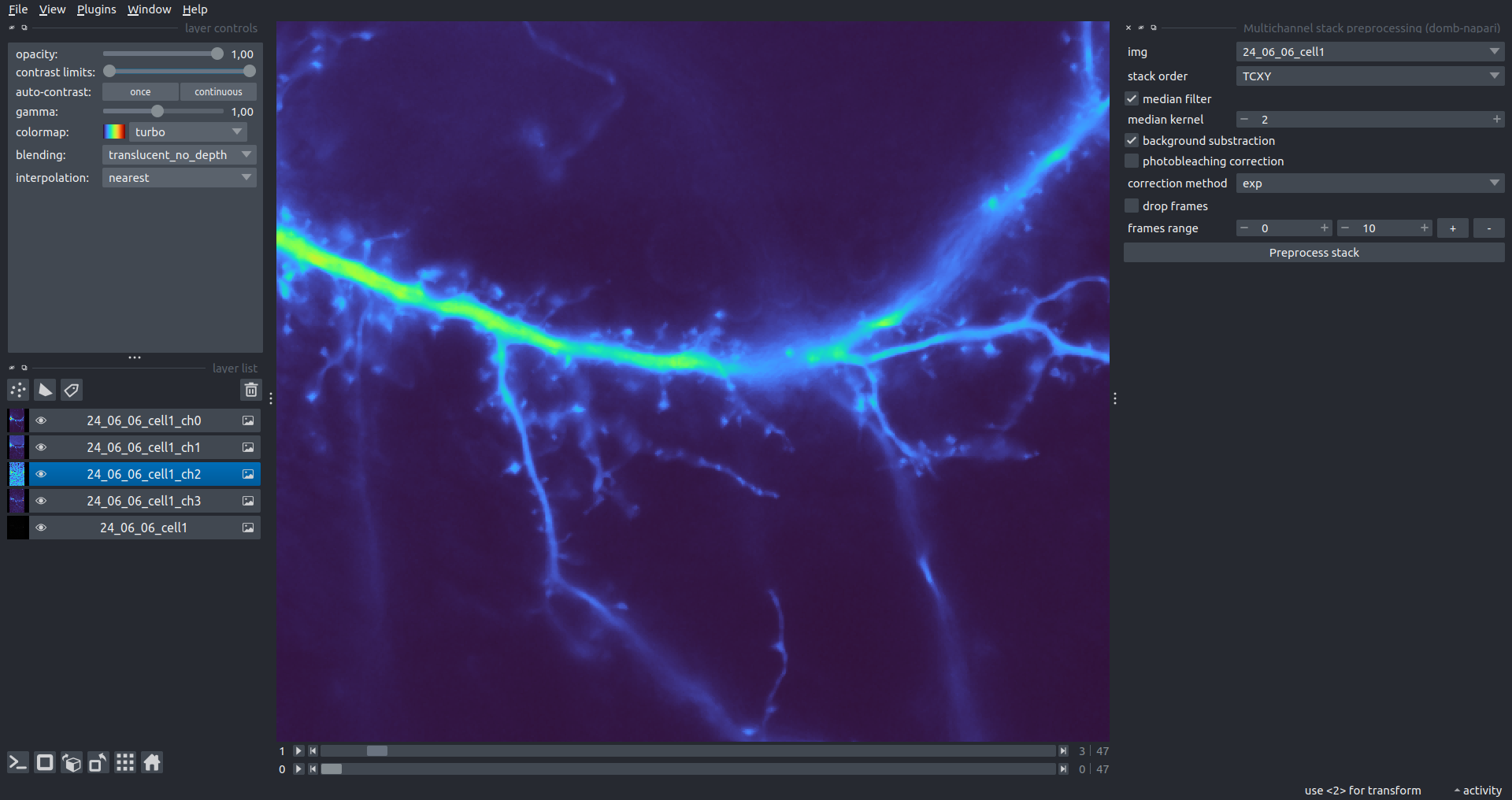\n\n---\n\n## Detection of Fluorescence Redistribution\nA set of widgets designed for preprocessing multispectral image stacks and detecting redistributions in fluorescence intensity. These widgets specifically analyze differential \"red-green\" image series to identify changes in fluorescence intensity.\n\nInspired by [Dovgan et al., 2010](https://pubmed.ncbi.nlm.nih.gov/20704590/) and [Osypenko et al., 2019](https://www.sciencedirect.com/science/article/pii/S0969996119301974?via%3Dihub).\n\n### Red-Green Series\nPrimary method for detecting fluorescence-labeled targets redistribution. This widget returns a series of differential images, each representing the intensity difference between the current frame and the previous one, output image labeled with the `_red-green` suffix.\n\nParameters:\n\n- `left frames` - specifies the number of previous frames used for pixel-wise averaging.\n- `space frames` - determines the number of frames between the last left frame and the first right frame.\n- `right frames` - specifies the number of subsequent frames used for pixel-wise averaging.\n\n`normalize by int` function normalizes the differential images relative to the absolute intensity of the input image stack, which helps to reduce background noise amplitude.\n\nIf `save MIP` is selected, the maximal intensity projection (MIP) of the differential image stack will be saved with the `_red-green-MIP` suffix.\n\n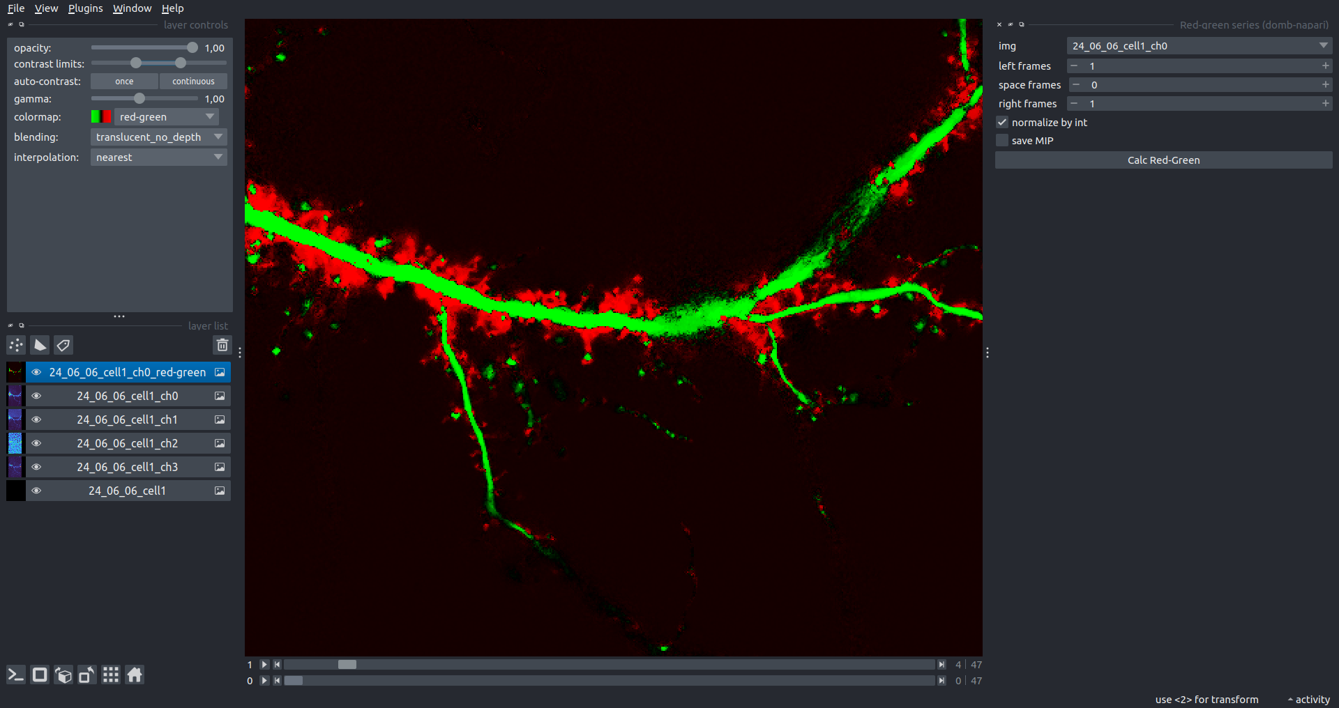\n\n### ΔF Series\nCalculates relative intensity changes for time-lapse images.\n\nParameters:\n\n- `values mode` - detection mode:\n - `ΔF` - absolute intensity changes ($F(t) - F_{0}$).\n - `ΔF/F0` - relative intensity changes ($(F(t) - F_{0}) / F_{0}$).\n- `F0 win` - window size (number of frames) for baseline intensity ($F_{0}$) estimation.\n\n---\n\n## Masking\n### Dots Pattern Masking\nCreates labels for bright dot elements on an image, such as pre- and postsynaptic fluorescence markers (e.g., Bassoon/Synaptobrevin for presynapses, PSD-95/Homer for postsynapses, etc.). It returns a labels layer with the `_dots-labels` suffix.\n\nThe widget detects the location on the MIP (Maximum Intensity Projection) of the input time series image and applies simple round masks to each detected dot. Watershed segmentation is then used to prevent the merging of overlapping masks.\n\nParameters:\n\n- `background level` - Background level for filtering out low-intensity elements. This is specified as a percentile of the MIP intensity.\n- `detection level` - Minimum intensity of dots, specified as a percentile of the MIP's maximum intensity.\n- `mask diameter` - Diameter in pixels for the round mask of each individual dot.\n- `minimal distance` - Minimum distance in pixels between the centers of individual round masks.\n\n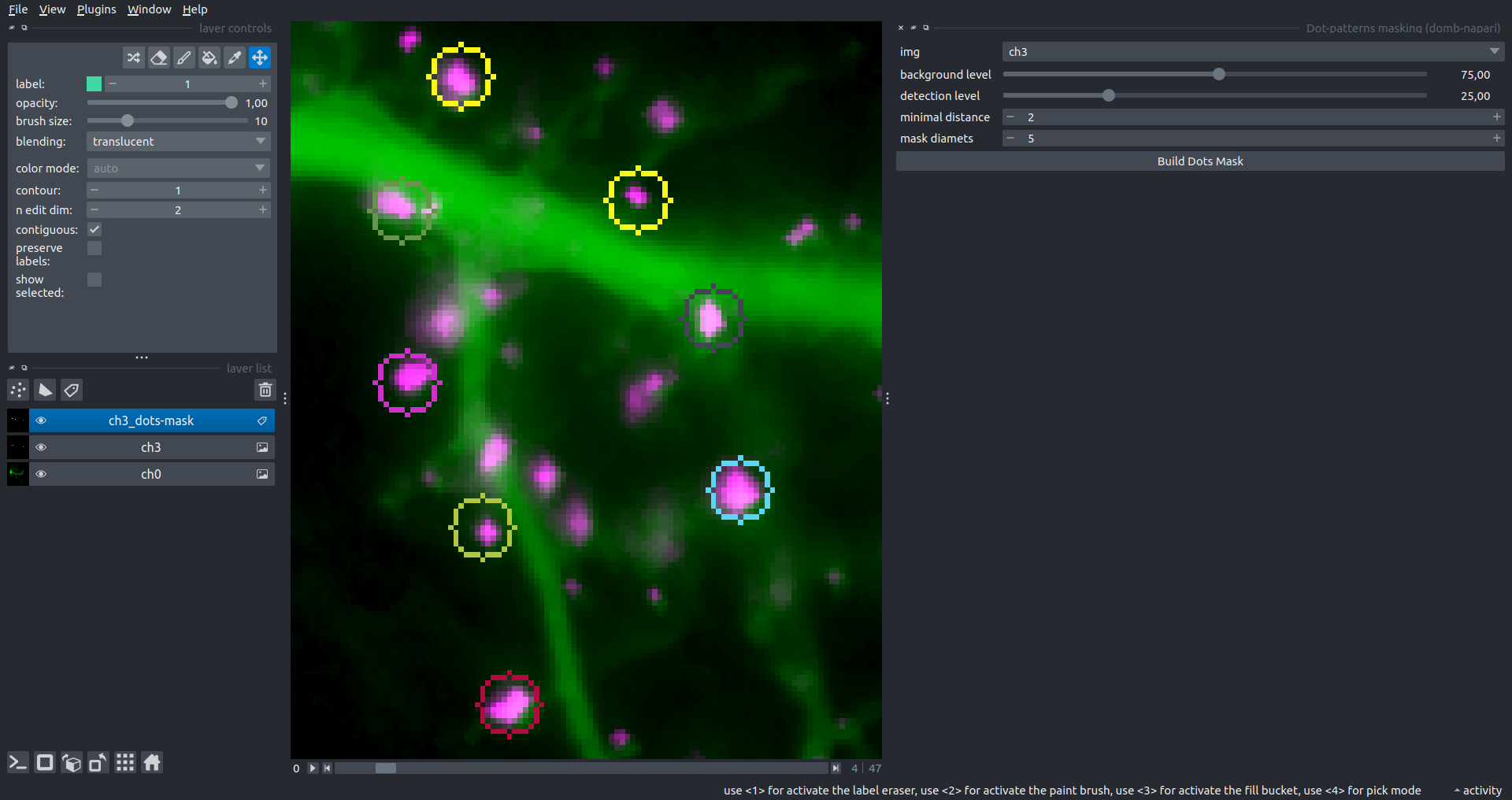\n__Hippocalcin (green) and PSD95 (magents) in dendritic branches__\n\n\n### Up Masking\nGenerates labels for regions with high intensity based on raw or -red-green images. Returns a labels layer with the `_up-labels` suffix.\n\nThe widget provides two detection modes:\n\n- Global masking with a fixed threshold for the entire image.\n- In-ROIs masking with a loop over individual ROIs in the input `ROIs mask` with separate detections.\n\nParameters:\n\n- `det frame index` - index of the frame from the input image used for label detection.\n- `det th` - threshold value for detecting bright sites, where the intensity on the selected frame is normalized in the range of -1 to 0.\n- `in ROIs det` - option for activating in-ROIs masking.\n- `in ROIs det method` - method for in-ROIs masking; otsu provides simple Otsu thresholding, while the threshold method is identical to global detection on normalized detection frame.\n- `in_ROIs_det_th_corr` - scaling factor for the det th threshold value for in-ROIs masking.\n- `final opening fp` - footprint size in pixels for mask filtering using morphological opening (disabled if set to 0).\n- `final dilation fp` - footprint size in pixels for mask morphological dilation (disabled if set to 0).\n- `save total up mask` - if selected, a total up mask (containing all ROIs) will be created with the _up-mask suffix.\n\n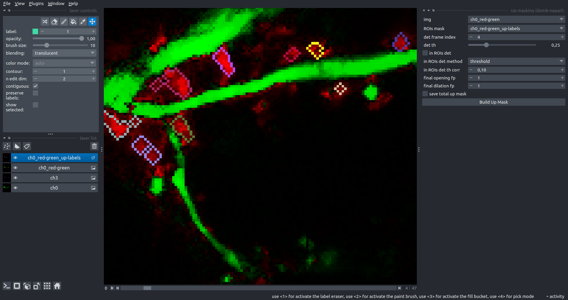\n__Global up labels__\n\nThe In-ROIs masking option can be particularly useful for co-localization detection. By applying a broad reference mask to several target images, you can create more precise labels for ROIs in specified cell compartments. The following examples demonstrate the detection of mutual locations for static PSD-95 enriched sites (postsynaptic membranes) and HPCA translocation sites only in the vicinity of synapses, using `_dots-labels` for PSD95-mRFP images.\n\n> [!IMPORTANT]\n> In the In-ROIs masking mode, labels of detected sites correspond to the matching labels from the input ROIs mask.\n\nIn-ROIs masking (reference)|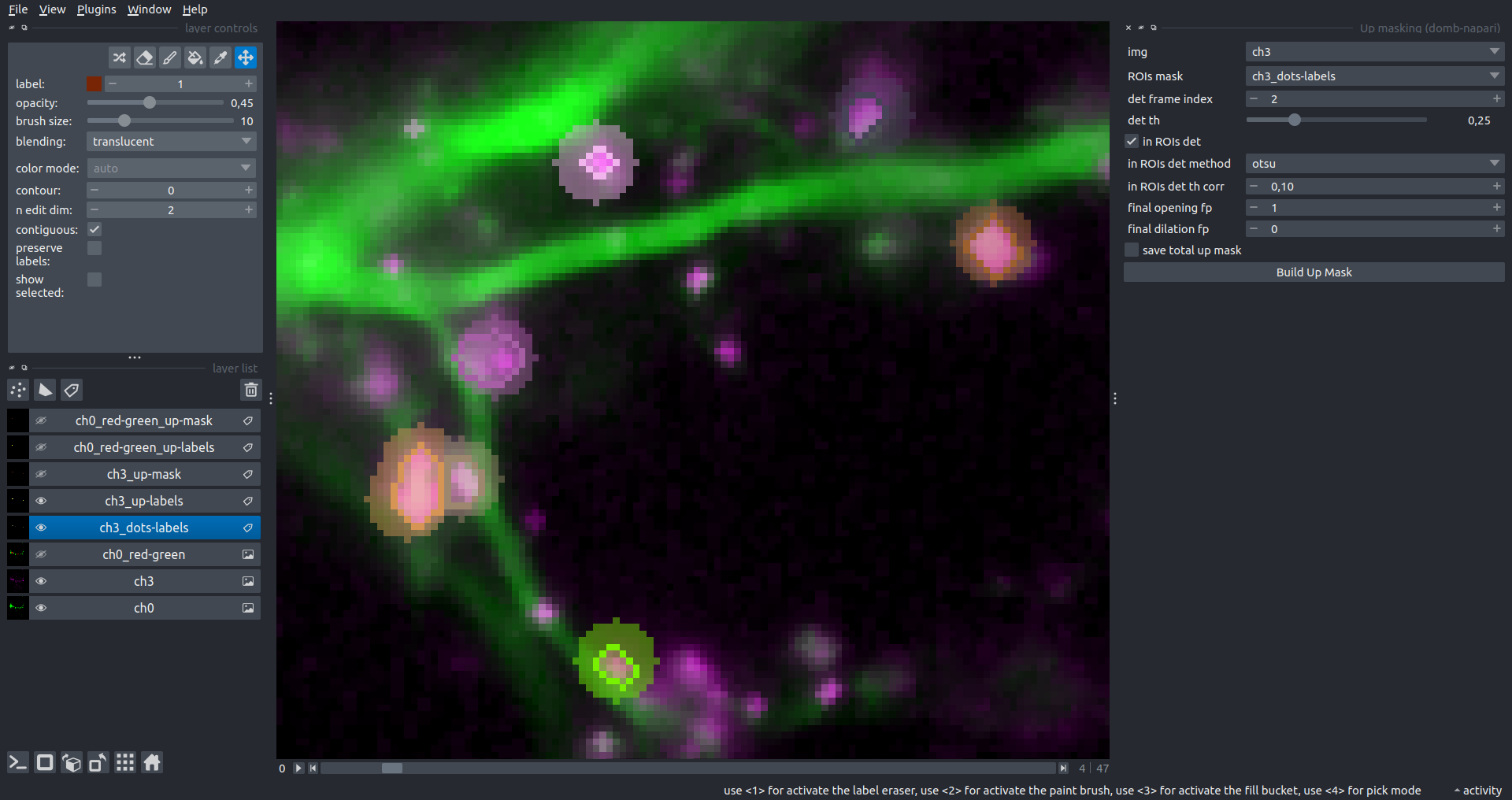\n:------------------:|:-------------------------:\n__In-ROIs masking (translocation)__|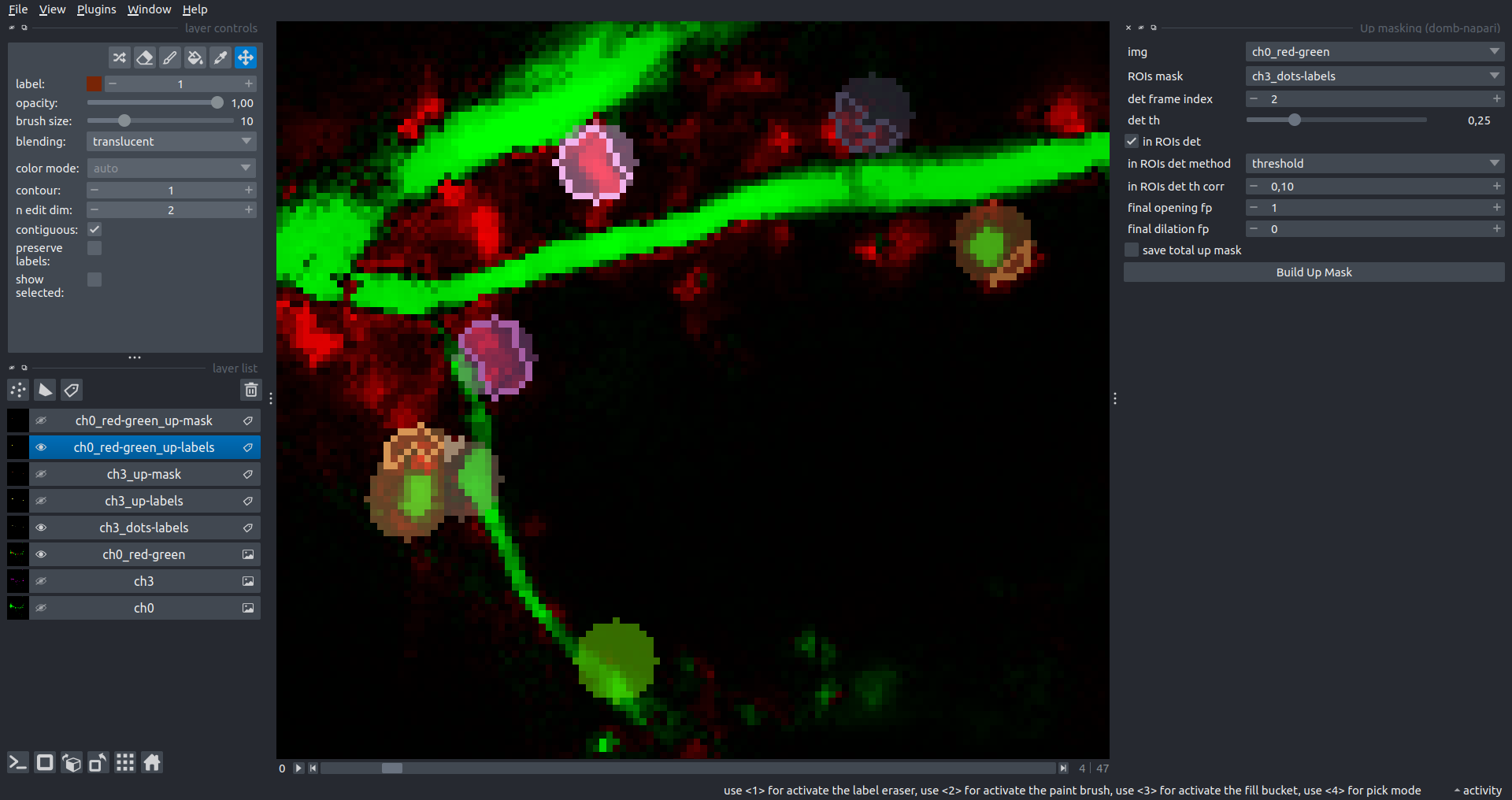\n__Masks overlay__|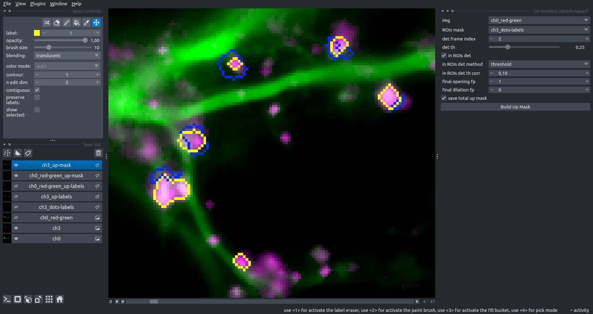\n\n\n### Intensity Masking\nExtension of the __Up Masking__ widget. Detects regions with either significantly increasing (`up`) or decreasing (`down`) intensity in `-red-green` differential images.\n\nParameters:\n\n- `masking mode` - defines whether to detect local intensity gains or losses.\n- `up threshold` - sensitivity for detecting intensity increases (normalized to maximum intensity).\n- `down threshold` - sensitivity for detecting intensity decreases.\n- `opening footprint` - disk radius for morphological opening to filter out noise.\n\n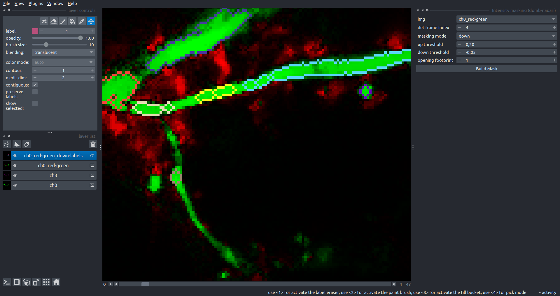\n\n---\n\n## 3-cube E-FRET Approach\nWidgets for detection and analysis of Förster resonance energy transfer on multispectral image stacks.\n\nBased on notation and approaches from [Zal and Gascoigne, 2004](https://pubmed.ncbi.nlm.nih.gov/15189889/), [Chen et al., 2006](https://pubmed.ncbi.nlm.nih.gov/16815904/) and [Kamino et al., 2023](https://pubmed.ncbi.nlm.nih.gov/37014867/).\n\n\n### E-FRET Cross-talk Estimation\nEstimates the cross-talk/bleed-through of fluorescence between the donor and acceptor’s spectral channels. \n\n```math\nF_c = I_{DA} - a (I_{AA} - c I_{DD}) - d (I_{DD} - b I_{AA})\n```\n\n```math\nF_c = I_{DA} - a I_{AA} - d I_{DD} \\; \\text{if} \\; b \\approx c \\approx 0\n```\n\n```math\na = \\frac{I_{DA(A)}}{I_{AA(A)}}\n```\n\n```math\nb = \\frac{I_{DD(A)}}{I_{AA(A)}}\n```\n\n```math\nc = \\frac{I_{AA(D)}} {I_{DD(D)}}\n```\n\n```math\nd = \\frac{I_{DA(D)}} {I_{DD(D)}}\n```\n\n```math\nb \\approx c \\approx 0\n```\n\nParameters:\n- `DD img` - $I_{DD}$, donor emission channel image acquired with the donor excitation wavelength.\n- `DA img` - $I_{DA}$, donor emission channel image acquired with the acceptor excitation wavelength.\n- `AD img` - $I_{AD}$, acceptor emission channel image acquired with the donor excitation wavelength.\n- `AA img` - $I_{AA}$, acceptor emission channel image acquired with the acceptor excitation wavelength.\n- `mask` - labels layer used for masking cellular regions.\n- `presented_fluorophore` - specifies the fluorophore present in the sample (`A` for Acceptor, `D` for Donor).\n- `saving_path` - directory where the output CSV file with coefficients will be saved.\n\n\n### E-FRET G-factor Estimation\nEstimates the G-factor using high and low FRET samples. Supports methods by [Zal and Gascoigne, 2004](https://pubmed.ncbi.nlm.nih.gov/15189889/) and [Chen et al., 2006](https://pubmed.ncbi.nlm.nih.gov/16815904/). \n\n```math\nG = \\frac{(I_{DA} - a I_{AA} - d I_{DD}) - (I_{DA}^{post} - a I_{AA}^{post} - d I_{DD}^{post})}{I_{DD}^{post} - I_{DD}} = \\frac{F_c - F_{c}^{post}}{I_{DD}^{post} - I_{DD}} = \\frac{\\Delta F_C}{\\Delta I_{DD}}\n```\n\n\n```math\n\\Delta F_c = G \\cdot \\Delta I_{DD}\n```\n\nParameters:\n\n- `estimation method` - method for G-factor estimation:\n - `Zal` - linear regression of $\\Delta F_c$ vs $\\Delta I_{DD}$ (Zal & Gascoigne, 2004).\n - `Chen` - intersection of lines from high and low FRET samples (Chen et al., 2006).\n- `DD img high FRET` / `low FRET` - $I_{DD}$ images for high and low FRET samples.\n- `DA img high FRET` / `low FRET` - $I_{DA}$ images for high and low FRET samples.\n- `AA img high FRET` / `low FRET` - $I_{AA}$ images for high and low FRET samples.\n- `mask` - (for `Zal` method) labels layer for ROIs.\n- `segment mask` - (for `Zal` method) if enabled, automatically segments the mask into smaller ROIs.\n- `mask high` / `mask low` - (for `Chen` method) masks for high and low FRET samples.\n- `a` & `d` - pre-calculated cross-talk coefficients.\n- `saving_path` - directory where the output CSV file with G-factor data will be saved.\n\n### E-FRET Estimation\nEstimation of the E-FRET with 3-cube approach.\n\n```math\nE_{D} = \\frac{F_c / G}{F_c / G + I_{DD}}\n```\n\nParameters:\n\n- `Сonfig mode` - source of FRET coefficients:\n - `Default` - uses pre-defined coefficients from the plugin directory.\n - `Load` - allows selecting a custom YAML configuration file via `config path`.\n- `fret pair` - selects the specific fluorophore pair (from the loaded configuration).\n- `DD img` - donor emission channel image (donor excitation).\n- `DA img` - acceptor emission channel image (donor excitation).\n- `AA img` - acceptor emission channel image (acceptor excitation).\n- `output type` - output image type:\n - `Fc` - sensitized emission (cross-talk corrected).\n - `E_D` - donor-centric apparent FRET efficiency (Zal and Gascoigne, 2004).\n - `E_A` - acceptor-centric FRET ratio (Erickson et al., 2001).\n - `Ecorr` - FRET efficiency corrected for acceptor photobleaching.\n- `save normalized` - if enabled, saves an additional image normalized to the absolute intensity of the `AA img`.\n\n> [!WARNING]\n> Normalized images are intended for visual inspection and mask construction only; they should not be used for quantitative analysis.\n\nRaw Eapp| 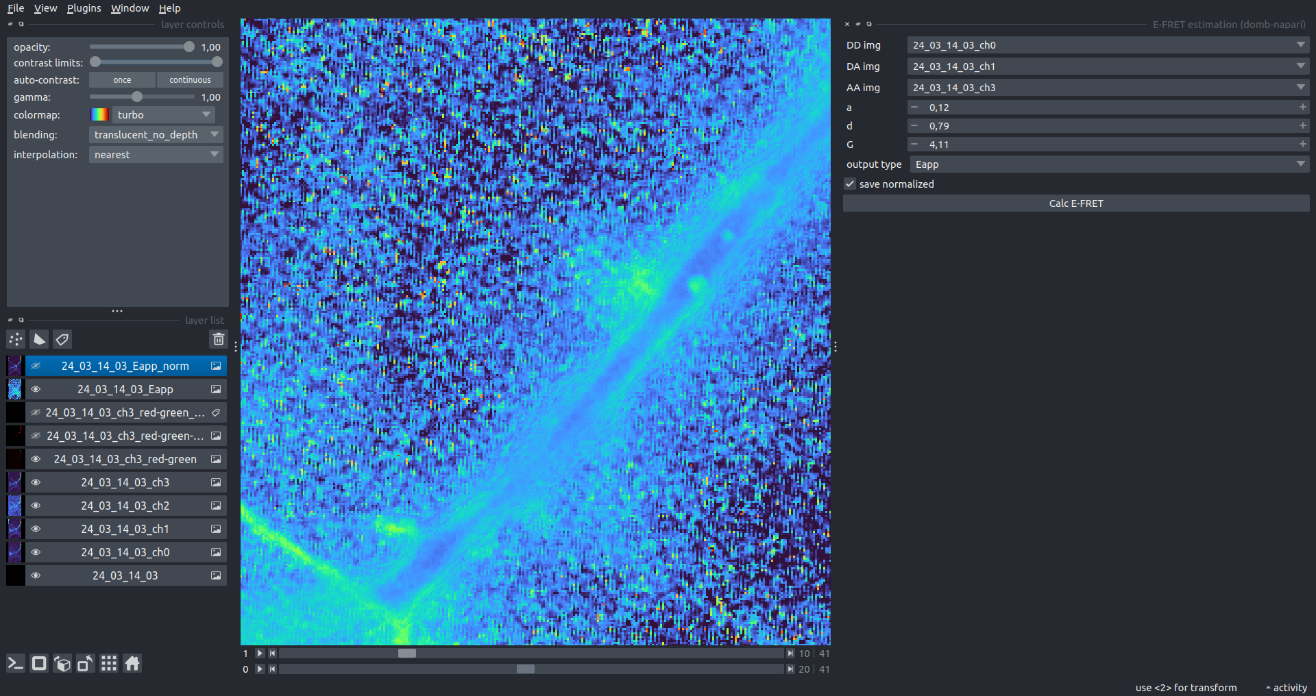\n:-:|:-:\n__Normalized Eapp__|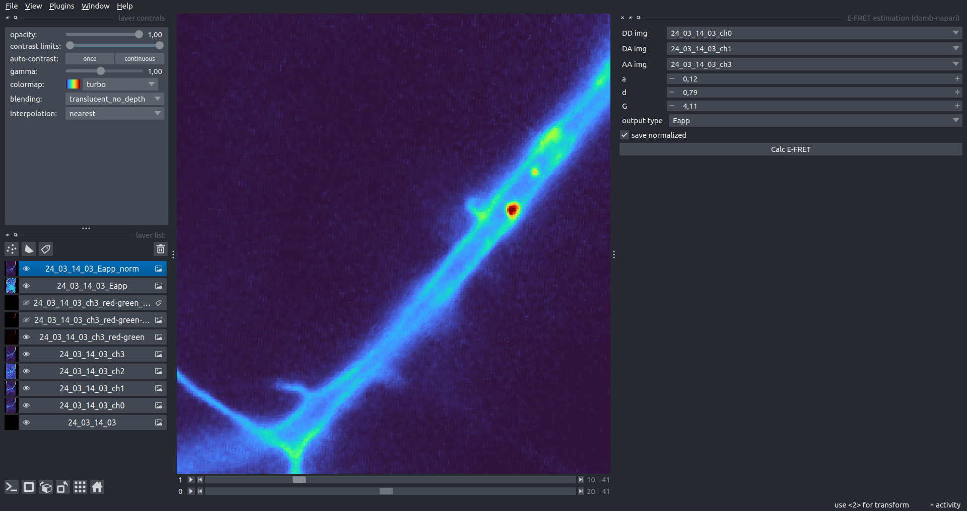\n\n\n### FRET Coefficients Configuration\nThe plugin uses a YAML configuration file to store and load coefficients for different FRET pairs. By default, it uses `_e_fret_coefs.yaml` located in the plugin directory.\n\nThe configuration file structure:\n\n```yaml\nFRET_Pair_Name:\n a: 0.031 # Acceptor cross-talk coefficient (I_DA(A) / I_AA(A))\n d: 0.415 # Donor cross-talk coefficient (I_DA(D) / I_DD(D))\n G: 9.26 # Gauge (G) factor\n xi: 0.0535 # Ratio of acceptor/donor extinction coefficients (at donor excitation)\n```\n\nUsers can provide a custom configuration file via the `E-FRET Estimation` widget by switching the `Config mode` to `Load`.\n\n\n### Stand-alone E-FRET Module\nThe core FRET logic is implemented in the stand-alone module `_e_fret.py`. This module can be used independently of the napari interface for batch processing or custom analysis scripts.\n\nKey classes in `_e_fret.py`:\n\n- `CubesFRET` - basic class for FRET estimation. Supports calculation of sensitized emission ($F_c$), apparent FRET efficiency ($E_D$), FRET ratio ($E_A$), and corrected FRET efficiency ($E_{corr}$).\n- `CrossTalkEstimation` - estimates $a$ and $d$ coefficients using linear regression of pixel intensities from single-fluorophore reference samples.\n- `GFactorEstimation` - estimates the $G$-factor using either the acceptor photobleaching method ([Zal and Gascoigne, 2004](https://pubmed.ncbi.nlm.nih.gov/15189889/)) or the multi-FRET-level method ([Chen et al., 2006](https://pubmed.ncbi.nlm.nih.gov/16815904/)).\n- `KFactorEstimation` - estimates the $k$ factor used for donor/acceptor concentration ratio calculations.\n\nThe module utilizes `numba` JIT compilation for high-performance pixel-wise calculations and `pandas`/`scipy` for statistical analysis during calibration steps.\n\n---\n\n## Plotting and Data Frame Saving\n### ROIs Profiles\nThis widget builds a plot with mean intensity profiles for each Region of Interest (ROI) in labels. It uses either absolute intensity (if `absolute intensity` is selected) or relative intensities (ΔF/F0).\n\nParameters:\n\n- `time scale` - sets the number of seconds between frames for x-axis scaling.\n- `values mod` - the mode of output profile calculation. Options are `ΔF/F0` (relative intensity changes), `ΔF` (absolute intensity changes), or `abs` (absolute intensity value)\n- `ΔF win`: if the `use_simple_baseline` option is selected, the baseline is the mean of the initial profile points. Otherwise, it defines the median filter window for the `pybaselines` estimator.\n- `Dietrich std`: (for `pybaselines` only) the number of standard deviations for thresholding in the Dietrich method.\n- `profiles crop` - crops the plotted profiles to the specified `profiles range`.\n\nAbsolute intensity | 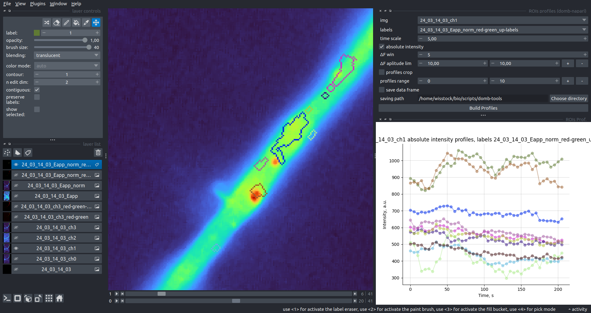\n:-------------------------:|:-------------------------:\n__ΔF/F0__|\n\n\n### Multiple Images Stat Profiles\nThis widget builds a plot displaying the average intensity of all Regions of Interest (ROIs) specified in `lab`. It can handle up to three images (`img 0`, `img 1`, and `img 2`) as inputs, depending on the selected `profiles num`.\n\n`time scale`, `values mod`, and `ΔF win` parameters are identical as described in the __ROIs profiles__ widget.\n\nThe `stat method` allows estimation of intensity and associated errors using the following methods:\n- `se` - mean ± standard error of the mean.\n- `iqr` - median ± interquartile range.\n- `ci` - mean ± 95% confidence interval (t-distribution).\n\nAbsolute intensity | 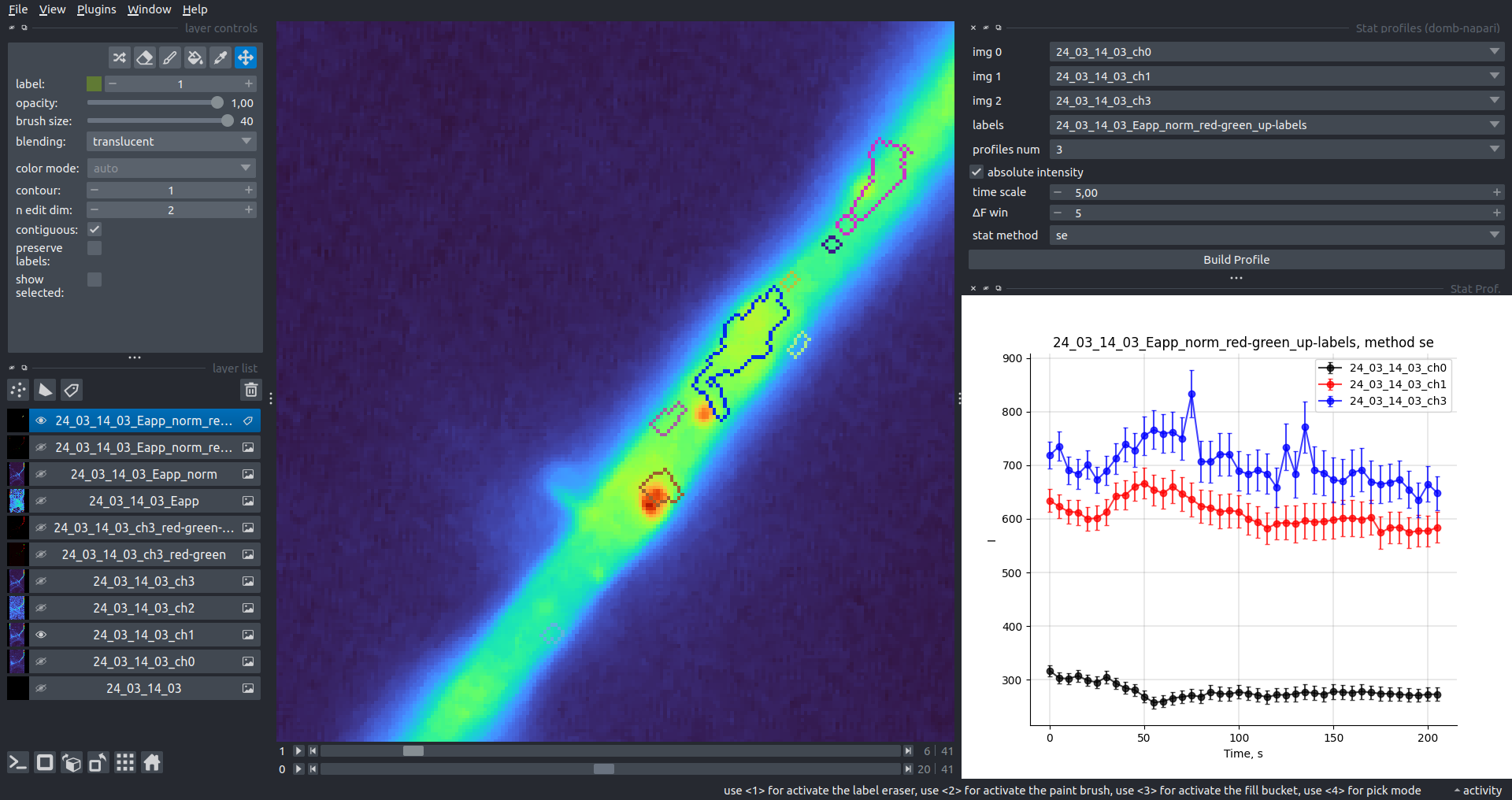\n:-------------------------:|:-------------------------:\n__ΔF/F0__|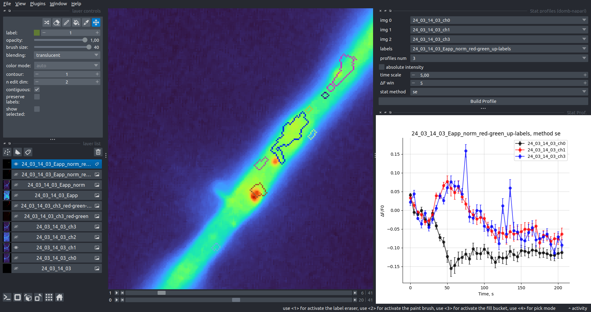\n\n\n### Multiple Labels Stat Profiles\nThis widget builds a plot displaying the averaged intensity of all Regions of Interest (ROI) for one target `img`. It can handle up to three labels (`lab 0`, `lab 1`, and `lab 2`), depending on the selected `profiles num`.\n\n`time scale`, `values mod`, and `ΔF win` parameters are identical as described in the __ROIs profiles__ widget.\n\nThe `stat method` allows estimation of intensity and associated errors using the following methods:\n- `se` - mean +/- standard error of the mean.\n- `iqr` - median +/- interquartile range.\n- `ci` - mean +/- 95% confidence interval based on the t-distribution.\n\nAbsolute intensity | 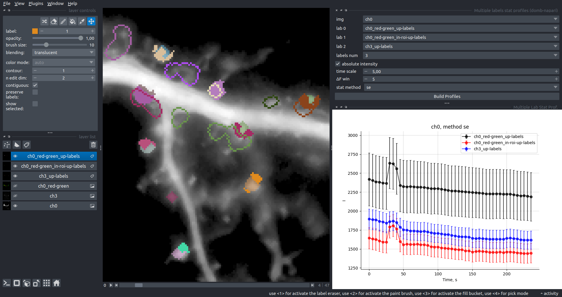\n:-------------------------:|:-------------------------:\n__ΔF/F0__|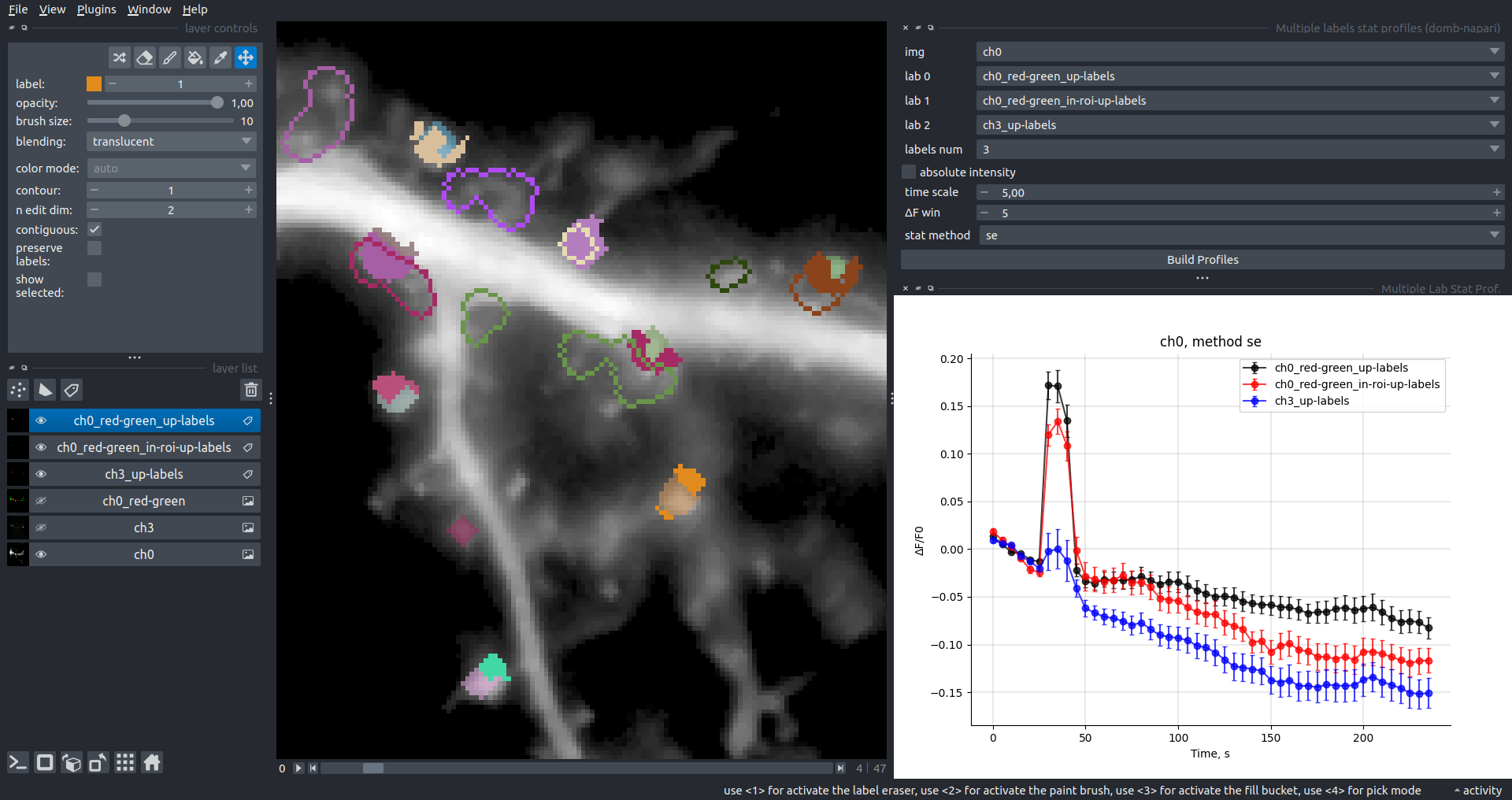\n\n### Save Data Frame\nThis widget enables you to save the data frame in CSV format.\nThis is particularly useful for exporting results after examining them with the __ROIs Profiles__ widget.\n\nParameters:\n\n- `img` - input for a single channel time series image stack.\n- `lab` - input for a labels layer with ROIs.\n- `stim position` - input for a points layer with stimulation electrode position, should contain a single point only.\n- `time scale` - input for frame-to-seconds scaling.\n- `ΔF win`: baseline window for the simple estimator.\n- `Dietrich win` & `Dietrich std`: window size and threshold for the `pybaselines` Dietrich estimator.\n- `save ROIs distances` - calculates and saves the average distance (pixels) from ROIs to a stimulation point.\n- `custom stim position` - uses a point from the `stim position` layer for distance calculations.\n\nThe output CSV contains:\n- `id` & `lab_id`: source Image and Labels layer names.\n- `roi`: ROI index.\n- `dist`: average distance to stimulation point (if enabled).\n- `index` & `time`: frame indices and timestamps.\n- `abs_int`, `dF_int`, `dF/F0_int`: absolute, differential, and relative intensities.\n- `base`: the baseline estimation method used (`simple` or `dietrich`).\n\n---\n\n## How to Cite\nIf you use this plugin in your work, please cite the following paper:\n\n```\n@article{Olifirov2025,\n title = {Local Iontophoretic Application for Pharmacological Induction of Long-Term Synaptic Depression},\n volume = {15},\n ISSN = {2331-8325},\n url = {http://dx.doi.org/10.21769/BioProtoc.5338},\n DOI = {10.21769/bioprotoc.5338},\n number = {1373},\n journal = {BIO-PROTOCOL},\n publisher = {Bio-Protocol, LLC},\n author = {Olifirov, Borys and Fedchenko, Oleksandra and Dovgan, Alexandr and Babets, Daria and Krotov, Volodymyr and Cherkas, Volodymyr and Belan, Pavel},\n year = {2025}\n}\n```\n\nor zenodo:\n```\n@misc{https://doi.org/10.5281/zenodo.14843770,\n doi = {10.5281/ZENODO.14843770},\n url = {https://zenodo.org/doi/10.5281/zenodo.14843770},\n author = {wisstock, },\n title = {wisstock/domb-napari: Zenodo release v0.3.0},\n publisher = {Zenodo},\n year = {2025},\n copyright = {MIT License}\n}\n```\n","description_content_type":"text/markdown","keywords":null,"home_page":null,"download_url":null,"author":null,"author_email":"Borys Olifirov ","maintainer":null,"maintainer_email":null,"license":null,"classifier":["Framework :: napari","Development Status :: 3 - Alpha","Programming Language :: Python :: 3.10","Programming Language :: Python :: 3.11","Programming Language :: Python :: 3.12","Programming Language :: Python :: 3.13","Operating System :: OS Independent","Topic :: Scientific/Engineering :: Bio-Informatics","Topic :: Scientific/Engineering :: Image Processing","Topic :: Scientific/Engineering :: Visualization","Topic :: Utilities"],"requires_dist":["napari","dipy","numpy","scipy","scikit-image","tifffile","pandas","matplotlib","numba","pybaselines"],"requires_python":">=3.10","requires_external":null,"project_url":["Homepage, https://github.com/wisstock/domb-napari","Documentation, https://github.com/wisstock/domb-napari","Repository, https://github.com/wisstock/domb-napari","BugTracker, https://github.com/wisstock/domb-napari/issues","Issues, https://github.com/wisstock/domb-napari/issues"],"provides_extra":null,"provides_dist":null,"obsoletes_dist":null},"npe1_shim":false}